Jekyll2026-11-11T09:14:52+00:00https://pnhuy.github.io/feed.xmlHuyNotesMy Learning Curve
Huy PhamAn Attention-Based Multi-Input Network for EGFR Inhibitors2026-08-25T00:00:00+00:002026-08-25T00:00:00+00:00https://pnhuy.github.io/machinelearning/2026/08/25/attention-multi-input-egfr-inhibitorsA few years after the Angel’s trumpet work,
I was doing the same kind of question — which molecules are active, and why — with a GPU instead of
a separatory funnel. This post introduces the paper I wrote with
Trung Hoang Le:
Attention-based Multi-Input Deep Learning Architecture for Biological Activity Prediction: An Application in EGFR Inhibitors
published at the 2019 11th International Conference on Knowledge and Systems Engineering (KSE).
Code is at lehgtrung/egfr-att.
The problem with training features separately
A molecule can be described two ways, and they carry different information.
You can describe its structure — the atoms, the bonds, the rings — usually as a fingerprint
vector or, as we did, straight from the SMILES string. Or you can describe its chemistry —
logP, dipole moment, the thousand-odd computed molecular descriptors that summarise how the
whole molecule behaves.
Studies had already established that combining both helps. But the way it was done was: train
one model on structure, train a second model on descriptors, then feed both outputs into a third
model that makes the final call. That works, and it is also awkward. Every feature set needs its
own algorithm, so you cannot build one pipeline; you build three and hope they stay in sync.
The models never see each other during training.
Our question was simply: what if both go into one network, trained at once?
The second problem was interpretation. A neural network that says 0.87, inhibitor and nothing
else is hard to use in medicinal chemistry, where the actionable question is which part of the
molecule you should keep and which part you should change.
The architecture
Two branches meeting at a concatenation.
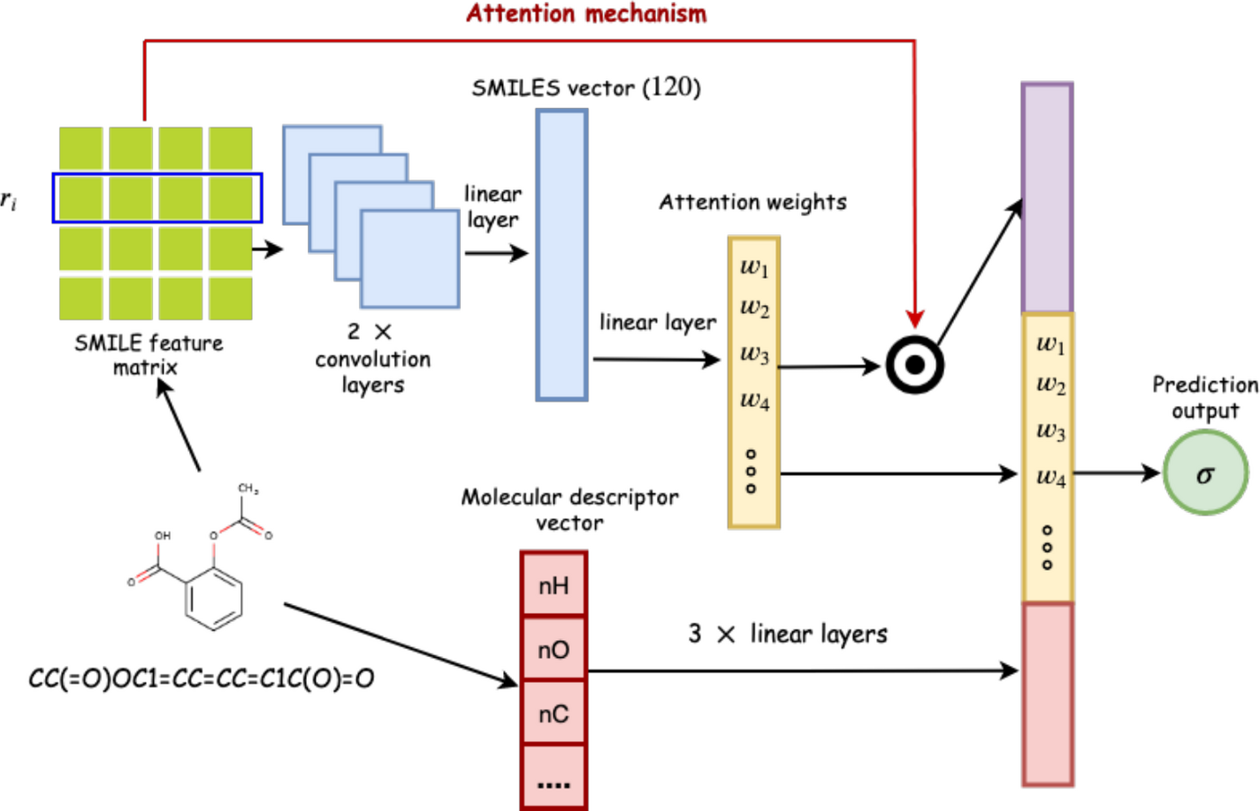
The CNN branch takes structure. Each SMILES string is encoded as a matrix using
M. Hirohara’s scheme: one row per character, padded to 150 rows, and 42 features per row — 21
describing the atom (element, attached hydrogens, degree, charge, valence, ring membership,
aromaticity, chirality, hybridisation) and 21 describing SMILES syntax (brackets, bonds,
branch markers, start and end). That matrix goes through two convolution blocks — conv2d, batch
norm, dropout, max pool — and a linear layer.
The MD branch takes chemistry. 1613 two-dimensional descriptors computed with mordred,
cleaned of constant and meaningless columns, standard-scaled, then three fully connected blocks
narrowing 512 → 128 → 64.
The attention layer sits on the structural branch. Let $R_i$ be row $i$ of the SMILES
feature matrix — that is, one atom — and $\vec{m}$ the vector coming out of the CNN branch’s
linear layer. The attention weight for that atom is the similarity between the two, squashed:
\[a_i = \frac{1}{1 + \exp(R_i \cdot \vec{m})}\]
and the layer’s output is the weighted sum $\vec{f} = \sum_i a_i R_i$.
The point is that $a_i$ is a number attached to a specific atom. You can read it off after
training and ask the model which atoms it was looking at.
Then $\vec{f}$, $\vec{m}$ and the descriptor vector $\vec{t}$ are concatenated, passed
through one linear layer, and squashed by a sigmoid into the probability that the compound
inhibits EGFR.
The data
EGFR — the epidermal growth factor receptor — is a tyrosine kinase whose dysregulation drives
several cancers, lung cancer especially, which makes it one of the most-studied targets in
oncology.
We used H. Singh et al.’s dataset: 3492 compounds labelled inhibitor or non-inhibitor at an
IC50 threshold of 10 nM. The ratio is 506 inhibitors to 2986 non-inhibitors, about
1 : 6, so the class imbalance is real and the metric choice matters. Singh’s Random Forest model
on the same data is the baseline we had to beat.
Everything was implemented in PyTorch, tuned by grid search, and evaluated by 5-fold
cross-validation with early stopping at 30 epochs of rising loss. The winning configuration:
batch size 128, dropout 0.5, ADAM, learning rate 1e-5, decision threshold 0.2.
Results
We report MCC as the primary metric. Accuracy and F1 both ignore parts of the confusion matrix,
and on a 1 : 6 split that is how you fool yourself; MCC uses all four cells.
Metric
H. Singh et al.
CNN only
CNN + MD
CNN + MD + ATT
Sensitivity
69.89%
74.31%
75.29%
74.11%
Specificity
86.03%
85.77%
89.75%
90.15%
Accuracy
83.66%
84.10%
87.66%
87.83%
MCC
0.49
0.50
0.58
0.57
AUC
89.00%
87.52%
90.32%
90.84%
Loss
—
0.2727
0.2434
0.2399
Running time
—
59 min
31 min
37 min
Three things in that table are worth pulling out.
Structure alone is not enough. The CNN-only model barely matches the Random Forest baseline
and is actually worse on AUC. Our reading is sparsity: padding every SMILES string out to 150
rows leaves a mostly-empty matrix, and a sparse input needs more data than 3492 compounds to
train on.
Adding the descriptor branch fixes it. MCC goes 0.50 → 0.58, AUC 87.5% → 90.3%. The second
input gives the network information it can use immediately, rather than having to extract it
from a sparse matrix.
And it trains faster. The bigger model takes half the time of the small one — 31 minutes
against 59. The sparse-input model needs many more epochs to converge; when the descriptor
branch is there, information appears to flow between the branches and the loss settles much
sooner. That was the result that surprised us most, and it is exactly what the
train-each-feature-set-separately approach throws away.
What the model looks at
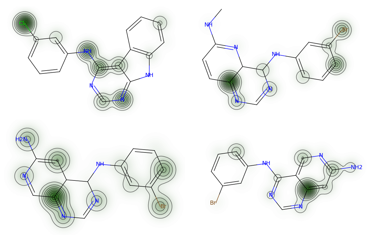
Attention weights, one per atom, rendered over the structure with rdkit. Darker means the
model weighted that atom more heavily.
Two patterns show up across compounds: nitrogens in heterocyclic rings are consistently
highlighted, and halobenzyl substitution on a heterocycle contributes positively to
predicted activity. Both are recognisable to anyone who has looked at this chemical series —
which is the point. The model is not being asked to teach us new pharmacology here; it is being
asked to show that its confidence rests on the parts of the molecule that ought to matter.
Note that attention cost us nothing on MCC (0.58 → 0.57) and gained a little on AUC and
specificity. We did not tune the attention model hard, because interpretability was what we
wanted from it.
Limitations
Attention is per-atom, so functional groups are invisible. Each row of the feature matrix is
one atom, weighted independently. A carbonyl or a carboxylic acid is a unit chemically, but the
model has no way to say so. The fix we proposed is a third branch embedding substructure
patterns — ECFP, or a hashed fingerprint — so groups can carry weight as groups.
The dataset is small for deep learning. 3492 compounds, and the CNN-only result shows what
that costs when the input is sparse.
Attention did not improve accuracy. It bought interpretation, not performance. Whether
tuning it properly would change that, we did not find out.
]]>Huy PhamTropane Alkaloids in Angel’s Trumpet Leaves2026-08-24T00:00:00+00:002026-08-24T00:00:00+00:00https://pnhuy.github.io/pharmacy/2026/08/24/tropane-alkaloids-in-angels-trumpet-leavesBefore any of the machine learning, I spent many years on a bench in Ho Chi Minh City taking a
plant apart. This was my thesis for my Degree of Pharmacist at the University of Medicine
and Pharmacy, supervised by Dr. Nguyen Viet Kinh and Mr. Nguyen Manh Tin Tin. I want to write it down properly, partly
because it is the work I am still most fond of, and partly because the reasoning in it —
find the one step that makes everything downstream easier — turned out to be the same
reasoning I use now on entirely different problems.
Brugmansia suaveolens, angel’s trumpet, is grown as an ornamental all over Vietnam. It is
a large, pleasant, drooping-flowered shrub that people plant next to their houses, and its
flowers and leaves have been eaten — sometimes deliberately, sometimes not. The poisonings
that follow have a particular character: dry mouth, dilated pupils, confusion, hallucination.
That is an anticholinergic syndrome, and it points at tropane alkaloids.
So there were two questions, one defensive and one opportunistic. Despite that people conducted
multiple studies on flower, the leaf had limited attention. What is actually in the
leaf that makes it poisonous? And given that whatever is in there is present in quantity,
could the leaf serve as a raw material for scopolamine?
The material
Twenty kilograms of dried leaf, collected at Di Linh in Lâm Đồng in March 2014, from the
yellow-flowered variety, ground to about 1×1 mm.
The separation
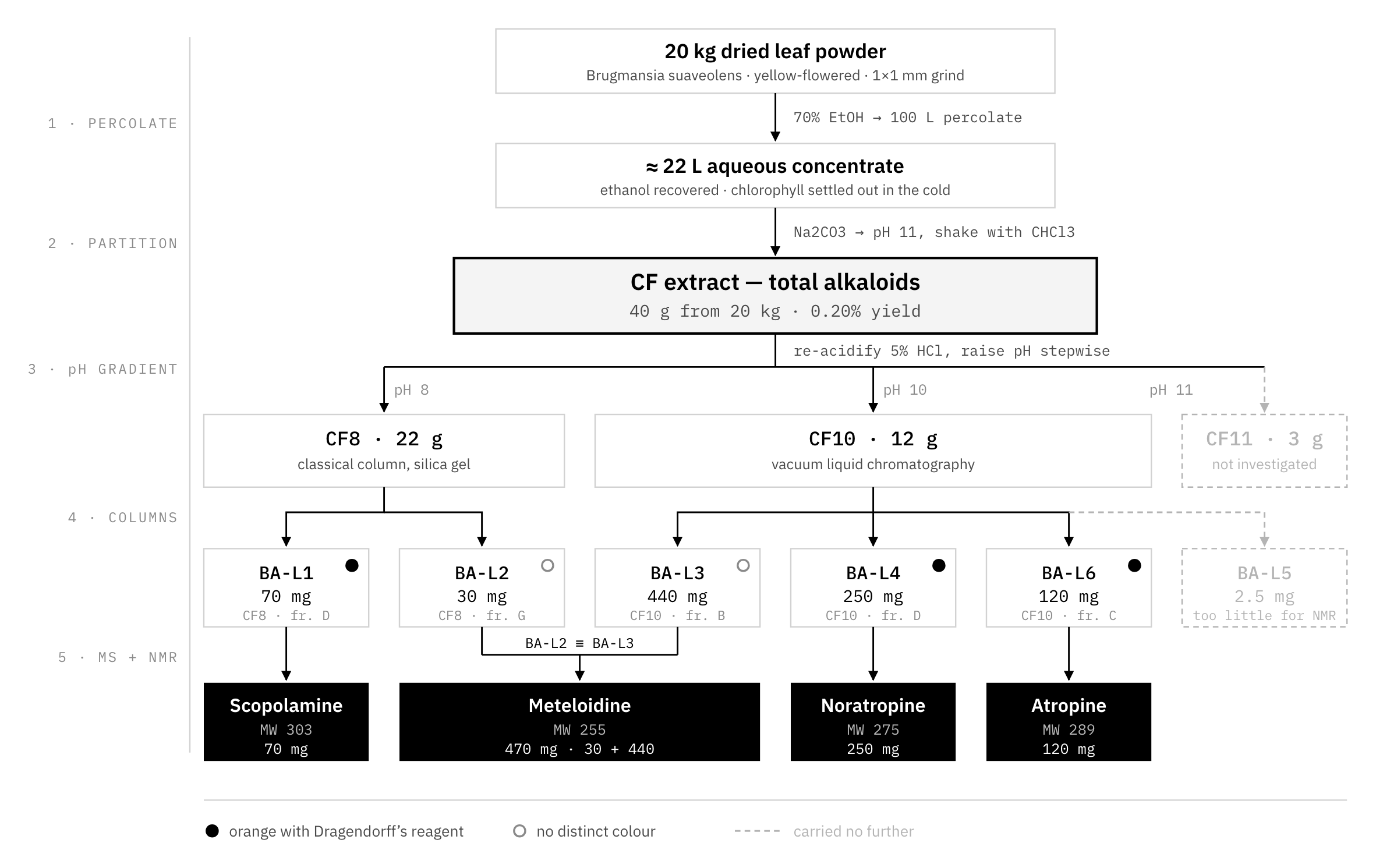
The whole scheme is below. It is worth reading before the commentary.
Percolation with 100 L of 70% ethanol, then the ethanol recovered and the concentrate left
in the cold so the chlorophyll would settle out — roughly 22 L of aqueous concentrate.
Basifying that to pH 11 with Na2CO3 and shaking against chloroform
gave 40 g of total alkaloid extract from 20 kg of leaf, a 0.20% yield.
Then the step the rest of the work rests on. Rather than take 40 g of mixed alkaloids
straight onto a column, I re-acidified with 5% HCl and raised the pH back up in stages,
extracting at each stop:
Fraction
pH
Mass
Then
CF8
8
22 g
classical silica-gel column
CF10
10
12 g
vacuum liquid chromatography
CF11
11
3 g
not investigated
Alkaloids differ in basicity, so they cross back into the organic phase at different pH.
Sorting them that way first means each fraction going onto a column already has one
predominant compound in it, and the chromatography has far less to do. This is the pivot of
the thesis: a cheap, low-tech separation placed before the expensive one, so the expensive
one becomes easy.
Six isolates came off the columns. Two of them, BA-L2 from CF8 and BA-L3 from CF10, turned
out by TLC and NMR to be the same substance appearing in both fractions — 30 mg and 440 mg
of the same compound.
The four compounds
Structures were assigned from MS together with 1H, 13C, DEPT, HSQC and
HMBC, run on a Bruker Avance 500 at the Institute of Chemistry, Vietnam Academy of Science
and Technology in Hanoi.
Code
Compound
Formula
MW
Isolated
BA-L1
Scopolamine
C17H21NO4
303
70 mg
BA-L2 / L3
Meteloidine
C13H21NO4
255
470 mg
BA-L4
Noratropine
C16H21NO3
275
250 mg
BA-L6
Atropine
C17H23NO3
289
120 mg
BA-L5
not determined
—
—
2.5 mg
All four share the tropane skeleton.
What it established
The leaf is not incidentally toxic. Three of the four identified compounds — atropine,
scopolamine, noratropine — are anticholinergic tropane alkaloids, and they are there in
quantity. The reported poisonings are exactly what you would predict from this composition.
That is the answer to the defensive question, and it argues for public awareness about a
plant most people treat as decoration.
The pH-gradient partition is transferable. Partitioning at pH 8, 10 and 11 before
chromatography should work on other Vietnamese Solanaceae carrying this compound class.
Four reference NMR profiles, usable in reference-substance documentation for testing
raw material and finished products.
A supply signal. Recovery is high enough that the leaf is worth evaluating seriously as
a source of scopolamine and hyoscyamine.
What I left open
The honest part of any thesis is the list of things you ran out of time for.
The 3 g of CF11 was never worked up, so the most basic alkaloids in the leaf remain
unmapped. The 70 mg scopolamine figure is a floor, not an estimate — only 1 g of the
12.89 g of fraction D was ever converted to the salt, so the leaf holds considerably more
than that number suggests. BA-L5 was 2.5 mg, too little to run NMR on. And I found
Brugmansia versicolor growing in Nghệ An, which deserves the same treatment and never
got it.
Ngoc-Huy Pham. “Studies on chemical constituents from Angel’s trumpet leaves (Folium Brugmansiae)”. Thesis for the degree of Bachelor of Pharmacy, University of Medicine and Pharmacy at Ho Chi Minh City, 2015–2016. Supervisor: Viet-Kinh Nguyen, PhD. Spectroscopy performed at the Institute of Chemistry, Vietnam Academy of Science and Technology, Hanoi.
]]>Huy PhamIntroduction to Linear Algebra2021-05-28T00:00:00+00:002021-05-28T00:00:00+00:00https://pnhuy.github.io/2021/05/28/Introduction-to-Linear-AlgebraVector
A vector is an ordered list of number, for example:
$$
x = \begin{bmatrix}
x_1 \\ x_2 \\ \vdots \\ x_n
\end{bmatrix}
$$
If $x,y \in \mathbb{R}^n$, the vectors addition & substraction is defined by
$$
x \pm y
=
\begin{bmatrix}
x_1 \pm y_1 \\
x_2 \pm y_2 \\
\vdots \\
x_n \pm y_n
\end{bmatrix}
$$
If $x,y \in \mathbb{R}^n$, the vector multiply is defined by
$$
x * y
=
\begin{bmatrix}
x_1 \times y_1 \\
x_2 \times y_2 \\
\vdots \\
x_n \times y_n
\end{bmatrix}
$$
If $x,y \in \mathbb{R}^n$, the inner product or dot product is a number given by
$$
x^T y
=
\begin{bmatrix}
x_1 & x_2 & \dots & x_n
\end{bmatrix}
\begin{bmatrix}
y_1 \\ y_2 \\ \vdots \\ y_n
\end{bmatrix}
=\sum_{i=1}^{n}x_i y_i
$$
The transpose of a matrix $A \in \mathbb{R}^{m \times n}$ is $A^T \in \mathbb{R}^{m \times n}$ whose entries are given by
\[(A^T)_{ij} = A_{ji}\]
The properties of transpose:
$(A^T)^T=A$
$(AB)^T = B^T A^T$
$(A+B)^T = A^T + B^T$
Given a square matrix $A$, if $A = A^T$, A is said to be symmetric. It is anti-symmetric if $A = -A^T$.
For any square matrix $A$, the matrix $A + A^T$ is symmetric and the matrix $A-A^T$ is anti-symmetric.
The identity matrix $I \in \mathbb{R}^{n \times n}$ is a square matrix with ones on the diagonal and zeros everywhere else. For all $A \in \mathbb{R}^{m \times n}$, $AI = IA = A$
The inverse matrix of $A \in \mathbb{R}^{n \times n}$ is denoted $A^{-1}$ if and only if
$$A^{-1} A = A A^{-1} = I_n $$
If the inverse matrix of $A$ exists, A is invertible or nonsingular. Otherwise, if A has no inverse, A is singular or non-invertible.
For example, let
\(A =
\begin{bmatrix}
a & b \\
c & d
\end{bmatrix}\).
If $ad - bc \ne 0$, then A is invertible and
\[A^{-1} = \frac{1}{ad-bc}
\begin{bmatrix}
d & -b \\
-c & a
\end{bmatrix}\]
With two matrices $A \in \mathbb{R}^{m \times n}$ and $B \in \mathbb{R}^{n \times p}$, the product of A and B is the matrix $C \in \mathbb{R}^{m \times p}$ and \(C_{ij} = \sum^{n}_{k=1}A_{ik} B_{kj}\)
The product matrix only exists if the number of columns in $A$ equal to the number of rows in $B$.
For $n \ge 2$, the determinant of an $n \times n$ matrix $A = [a_{ij}]$ is the sum of $n$ terms of the form $\pm a_{1j} \det A_{1j}$, with plus and minus signs alternating, where the entries $a_{11}, a_{12}, \dots, a_{1n} $ are from the first row of $A$.
$$ \det A = |A| = a_{11} \det A_{11} - a_{12} \det A_{12} + \dots + (-1)^{1+n} a_{1n} \det A_{1n} $$
with $A_{ij}$ denotes the submatrix formed by deleting the $i$th row and $j$th column of A.
When the $(i,j)$-cofactor of A is the number $C_{ij}$ given by
$$ C_{ij} = (-1)^{i+j} \det A_{ij} $$
the determinant of A can be defined by
$$\begin{align}
\det A &= a_{i1} C_{i1} + a_{i2} C_{i2} + \dots + a_{in} C_{in} \\
&= a_{1j} C_{1j} + a_{2j} C_{2j} + \dots + a_{nj} C_{nj}
\end{align}$$
In the case $2 \times 2$ matrix:
\[\det
\begin{bmatrix}
a & b \\
c & b
\end{bmatrix}
=
\begin{vmatrix}
a & b \\
c & b
\end{vmatrix}
= ad - bc\]
and $3 \times 3$ matrix:
\[\begin{align}
\det
\begin{bmatrix}
a & b & c\\
d & e & f\\
g & h & i
\end{bmatrix}
&= a
\begin{vmatrix}
e & f \\
h & i
\end{vmatrix} -
b
\begin{vmatrix}
d & f \\
g & i
\end{vmatrix} +
c
\begin{vmatrix}
d & e \\
g & h
\end{vmatrix}\\
&= aei - afh -bdi +bfg + cdh - ceg
\end{align}\]
The determinant of the identity matrix is 1
\(\det I = \det \begin{vmatrix} 1 & 0 \\ 0 & 1 \end{vmatrix} = 1\)
The determinant changes sign when two rows are exchanged
\(\begin{vmatrix} c & d \\ a & b \end{vmatrix} = - \begin{vmatrix} a & b \\ c & d \end{vmatrix}\)
The determinant depends linearly on the first row
\(\begin{vmatrix} a+a' & b+b' \\ c & d \end{vmatrix} =
\begin{vmatrix} a & b \\ c & d \end{vmatrix} +
\begin{vmatrix} a' & b' \\ c & d \end{vmatrix}\)
\(\begin{vmatrix} ta & tb \\ c & d \end{vmatrix} =
t \begin{vmatrix} a & b \\ c & d \end{vmatrix}\)
If two rows of A are equal, then $\det A = 0$
\(\begin{vmatrix} a & b \\ a & b \end{vmatrix} = ab-ba = 0\)
Substracting a multiple of one row from another row leaves the same determinant
\(\begin{vmatrix} a- tc & b - td \\ c & d \end{vmatrix} =
\begin{vmatrix} a & b \\ c & d \end{vmatrix} - t \begin{vmatrix} c & d \\ c & d \end{vmatrix} = \begin{vmatrix} a & b \\ c & d \end{vmatrix}\)
If $A$ is triangular then $\det A$ is the product $a_{11} a_{22} \dots a_{nn}$ of the diagonal entries. If the triangular A has 1s , then $\det A = 1$
\(\begin{vmatrix} a & b \\ 0 & d \end{vmatrix} = \begin{vmatrix} a & 0 \\ c & d \end{vmatrix} = ad\)
If $A$ is singular, then $\det A = 0$. If $A$ is invertible, then $\det A \ne 0$
The determinant of AB is the product of $\det A$ times $\det B$: \(|A| |B| = |AB|\)
The special case is when $B = A^{-1}$:
\((\det A) (\det A^{-1}) = \det AA^{-1} = \det I = 1\)
\(\Rightarrow \det A^{-1} = \frac{1}{\det A}\)
The transpose of $A$ has the same determinant as $A$ itself: $\det A^T = \det A$
\(|A| = \begin{vmatrix} a & b \\ c & d \end{vmatrix} = \begin{vmatrix} a & c \\ b & d \end{vmatrix} = |A^T|\)
In case of 2 by 2 matrix, we have
\(\begin{bmatrix}
a & b \\
c & d \\
\end{bmatrix}
= \frac{1}{\det A}
\begin{bmatrix}
C_{11} & C_{21} \\
C_{12} & C_{22}
\end{bmatrix}
= \frac{1}{ad-bc}
\begin{bmatrix}
d & -b \\
-c & a
\end{bmatrix}\)
If $A$ is a $2 \times 2$ matrix, the area of the parallelogram determined by te columns of $A$ is $|\det A|$. If $A$ is a $3 \times 3$ matrix, the volume of the paralellepiped determined by the columns of $A$ is $|\det A|$.
Linear Independence
An set of vectors $\{ v_1, \dots , v_p \} \in \mathbb{R}^n$ is said to be linearly independent if the vector equation
$$ x_1 v_1 + x_2 v_2 + \dots + x_p v_p = 0 $$
has only the trivial solution.
The set $\{ v_1, \dots , v_p \} $ is said to be linearly dependent if there exist weights $c_1, \dots , c_p$, not all zero, such that
$$ c_1 v_1 + c_2 v_2 + \dots + c_p v_p = 0 $$
Rank
Given a matrix $A \in \mathbb{R}^{m \times n}$:
The column rank of $A$ is the size of the largest subset of columns of $A$ that constitute a linearly independent set.The row rank of $A$ is the size of the largest subset of rows of $A$ that constitute a linearly independent set
If the column rank of $A$ is equal to its row rank, this number is the rank of $A$.
The properties of the rank, for $A, B \in \mathbb{R}^{m\times n}$:
$rank(A) \le \min (m,n)$. If $rank(A) = \min(m,n)$, $A$ is said to be full rank.
$rank(A) = rank(A^T)$
$rank(AB) \le \min(rank(A), rank(B)$
$rank(A+B) \le rank(A) + rank(B)$
Norms
A norm is a function that satisfies the following three conditions:
Nonnegativity and mapping of the identity: if $x \ne 0$, then $\|x\| > 0$, and $\| 0 \|=0$
Scalar multiplication: $\| ax \| = |a| \| x\|$, for all real $a$
For $p \ge 1$, $L _ p$ norm is defined by
\(\| x \| _ {p} = \left( \sum_i \| x_i \|^p \right)^{\frac{1}{p}}\)
Some common $L_p$ norms:
$ | x |_ 1 = \sum _ {i} |x_i|$, also called the Manhattan norm.
$| x |_ 2 = \sqrt{\sum _ {i} x_i^2}$, also called the Euclidean norm, the Euclidean length, or the length of the vector. The $L_2$ is the square root of the inner product of the vector with itself: $|x|_ 2 = \sqrt{\langle x,x \rangle}$.
$| x |_ \infty = \max_{i} |x_i|$, also called the max norm or the Chebyshev norm.
A generalization of $L_p$ is the weighted $L_p$ norm:
\(\| x \|_ {wp} = \left(\sum_{i} w_i |x_i|^p \right)^{\frac{1}{p}}\)
Quadratic forms
A quadratic form in $\mathbb{R}^n$ is a function $Q$ defined on $\mathbb{R}^n$ whose value at a vector $x \in \mathbb{R}^n$ can be computed by an expression of the form $Q(x) = x^T Ax$, where $A$ is an $n \times n$ symmetric matrix. The matrix A is called the matrix of quadratic form.
$$
x^T Ax = \sum_{i=1}^{n}x_i (Ax)_i = \sum_{i=1}^{n}x_i \left( \sum_{j=1}^{n} A_{ij}x_{j}\right) = \sum_{i=1}^{n} \sum_{j=1}^{n} A_{ij} x_i x_j
$$
Positive definite and Positive semidefinite
Let A be symmetric matrix in $\mathbb{R}^n$:
A is positive definite if for all nonzero vectors $x\in \mathbb{R}^n$, $x^T Ax > 0$.
A is positive semidefinite if for all nonzero vectors $x\in \mathbb{R}^n$, $x^T Ax \ge 0$.
A is negative definite if for all nonzero vectors $x\in \mathbb{R}^n$, $x^T Ax < 0$.
A is negative semidefinite if for all nonzero vectors $x\in \mathbb{R}^n$, $x^T Ax \le 0$.
A is indefinite if A is neither positive semidefinite or negative semidefinite.
Eigenvalues and Eigenvectors
Given square matrix $A \in \mathbb{R}^{n \times n}$, we call that a scalar $\lambda$ is an eigenvalue of $A$ and a nonzero vector $x$ is the corresponding eigenvectr if $Ax = \lambda x$
How to find Eigenvalues and Eigenvectors?
Find the values of $\lambda$ which satisfy the characteristic equation:
\[\det (A- \lambda I) = 0\]
where $I$ is the identity matrix.
The solution of this equation is the eigenvalue of the matrix.
For each eigenvalue solved, we have
\[(A - \lambda I) x = 0\]
where x is the eigenvector associated with eigenvalue $\lambda$.
Find X by Gaussian elimination.
For example, find the eigenvalues and eigenvectors of
\(A=
\begin{bmatrix}
2 & -4 \\
-1 & -1
\end{bmatrix}\)
Solve the characteristic equation for eigenvalues:
[1] Lecture from course Machine learning at VEF Academy.
[2] Zico Kolter. Linear algebra review and reference, 2008.
[3] D.C. Lay, S.R. Lay, and J.J. McDonald. Linear Algebra and Its Applications. Pearson Education, 2015.
[4] G. Strang. Linear Algebra and Its Applications. Thomson, Brooks/Cole, 2006.
]]>Huy PhamIntroduction to Graph Theory2021-04-13T00:00:00+00:002021-04-13T00:00:00+00:00https://pnhuy.github.io/2021/04/13/Introduction-to-Graph-theoryGraph and Graph models
A graph $G=(V,E)$ consists of $V$, an nonempty set of vertices (or nodes) and $E$, a set of edges. Each edge has either one or two vertices associated with it, called its endpoints. An edge is said to connect its endpoints.
A graph with infinite vertex or egdes is called infinite graph. In the otherwise case, finite graph.
A graph in which each edge connects two different vertices and where no two edges connect the same pair of vertices is called a simple graph.
Graph that may have multiple edges connecting the same vertices are called multigraphs.
The edges that connect a vertex to itself are called loops.
Graphs including loops, and possibly multiple edges connecting the same pair of vertices or a vertex to itself, are called pseudographs.
The graph with undirected edges is an undirected graph.
A directed graph (or digraph) $(V,E)$ consists of a nonempty set of vertices $V$ and a set of directed edges (or arcs) $E$. Each directed edge is associated with an ordered pair of vertices. The directed edge associated with the ordered pair $(u,v)$ is said to start at $u$ and end at $v$.
A directed graph has no loops and has no multiple directed edges is called a simple directed graph.
Directed graphs that may have multiple directed edges from a vertex to a second (possibly the same) vertex are used to model such networks are called directed multigraphs. When there are $m$ directed edges, each associated to an ordered pair of vertices $(u,v)$, we say that $(u,v)$ is an edge of multiplicity $m$.
A graph with both directed and undirected edges is called a mixed graph.
Graphs are used in a wide variety of models:
Social networks
Communication networks
Information networks
Software design applications
Transportation networks
Biological networks
Tournaments
Terminology and special types of graph
Terminology
Two vertices u and v in an undirected graph G are called adjacent (or neighbors) in G if u and v are endpoints of an edge e of G. Such an edge e is called incident with the vertices u and v and e is said to connect u and v.
The set of all neighbors of a vertex v of $G=(V,E)$, denoted by $N(v)$, is called the neighborhood of $v$. If $A$ is a subset of $V$ , we denote by $N(A)$ the set of all vertices in $G$ that are adjacent to at least one vertex in A. So, $N(A)=\bigcup_{v\in A}N(v)$.
The degree of a vertex in an undirected graph is the number of edges incident with it, except that a loop at a vertex contributes twice to the degree of that vertex. The degree of the vertex v is denoted by $deg(v)$.
A vertex of degree zero is called isolated (not adjacent to any vertex).
A vertex is pendant if and only if it has degree one (adjacent to exactly one other vertex).
The handshaking theorem
Let $G=(V,E)$ be an undirected graph with $m$ edges:
$$2m=\sum_{v\in V}\deg(v)$$
This theorem shows that the sum of the degrees of the vertices of an undirected graph is even, which lead to the below theorem.
An undirected graph has an even number of vertices of odd degree.
When $(u,v)$ is an edge of the graph G with directed edges, $u$ is said to be adjacent to $v$ and $v$ is said to be adjacent from $u$. The vertex $u$ is called the initial vertex of $(u,v)$, and $v$ is called the terminal or end vertex of $(u,v)$. The initial vertex and terminal vertex of a loop are the same.
In a graph with directed edges the in-degree of a vertex v, denoted by $\deg^{-}(v)$, is the number of edges with v as their terminal vertex. The out-degree of v, denoted by $\deg^{+}(v)$, is the number of edges with v as their initial vertex. (Note that a loop at a vertex contributes 1 to both the in-degree and the out-degree of this vertex.)
Let $G=(V,E)$be a graph with directed edges:
$$\sum_{v\in V}\deg^{-}(v)=\sum_{v\in V}\deg^{+}(v)=|E|$$
Some special simple graphs:
Complete Graphs: a complete graph on n vertices, denoted by $K_{n}$, is a simple graph that contains exactly one edge between each pair of distinct vertices.
Wheels
n-cube / n-dimensional hypercube, denoted by $Q_{n}$, is a graph that has vertices representing the $2^{n}$ bit strings of length n.
Bipartite Graph
A simple graph $G$ is called bipartite if its vertex set $V$ can be partitioned into two disjoint sets $V_{1}$ and $V_{2}$ such that every edge in the graph connects a vertex in $V_{1}$ and a vertex in $V_{2}$ (so that no edge in $G$ connects either two vertices in $V_{1}$ or two vertices in $V_{2}$). When this condition holds, we call the pair $(V_{1},V_{2})$ a bipartition of the vertex set $V$ of $G$.
A simple graph is bipartite if and only if it is possible to assign one of two different colors to each vertex of the graph so that no two adjacent vertices are assigned the same color.
A complete bipartite graph $K_{m,n}$ is a graph that has its vertex set partitioned into two subsets of $m$ and $n$ vertices, respectively with an edge between two vertices if and only if one vertex is in the first subset and the other vertex is in the second subset.
A matching $M$ in a simple graph $G=(V,E)$ is a subset of the set $E$ of edges of the graph such that no two edges are incident with the same vertex. In other words, a matching is a subset of edges such that if ${s,t}$ and ${u,v}$ are distinct edges of the matching, then s, t, u, and v are distinct.
A vertex that is the endpoint of an edge of a matching $M$ is said to be matched in $M$; otherwise it is said to be unmatched.
A maximum matching is a matching with the largest number of edges. We say that a matching M in a bipartite graph $G=(V,E)$ with bipartition $(V_{1},V_{2})$ is a complete matching from $V_{1}$ to $V_{2}$ if every vertex in $V_{1}$ is the endpoint of an edge in the matching, or equivalently, if $|M|=|V_1|$.
Hall's marriage theorem / Necessary and sufficient conditions for complete matching
The bipartite graph $G=(V,E)$ with bipartition $(V_{1},V_{2})$ has a complete matching from $V_{1}$ to $V_{2}$ if and only if $\|N(A)\| \ge \|A\|$ for all subsets A of $V_{1}$.
Representing Graphs and Graph Isomorphism
Adjacency Lists
One way to represent a graph without multiple edges is to list all the edges of this graph. Another way to represent a graph with no multiple edges is to use adjacency lists, which specify the vertices that are adjacent to each vertex of the graph.
Adjacency Matrices
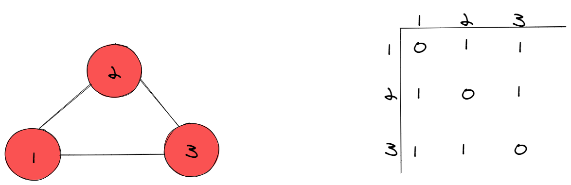
Suppose that $G = (V , E)$ is a simple graph where $|V| = n$. Suppose that the vertices of $G$ are listed arbitrarily as $v_1, v_2, …, v_n$ .
The adjacency matrix $A$ (or $A_G$ ) of $G$, with respect to this listing of the vertices, is the $n \times n$ zero–one matrix with 1 as its $(i, j)$th entry when $v_i$ and $v_j$ are adjacent, and 0 as its $(i,j)$th entry when they are not adjacent.
In other words, if its adjacency matrix is $A = [a_{ij}]$, then
\[a_{ij} = \left\{
\begin{matrix}
1 & \text{if } {v_i, v_j} \text{ is an edge of G} \\
0 & \text{otherwise}
\end{matrix}
\right.\]
Incidence Matrices
Let $G = (V , E)$ be an undirected graph. Suppose that $v_1 , v_2 , . . . , v_n$ are the vertices and $e1 , e2 , . . . , e_m$ are the edges of G. Then the incidence matrix with respect to this ordering of $V$ and $E$ is the $n \times m$ matrix $M = [m_{ij}]$, where
The simple graphs $G_1 = (V_1 , E_1 )$ and $G_2 = (V_2 , E_2 )$ are isomorphic if there exists a one-to-one and onto function $f$ from $V_1$ to $V_2$ with the property that $a$ and $b$ are adjacent in $G_1$ if and only if $f(a)$ and $f(b)$ are adjacent in $G_2$ , for all $a$ and $b$ in $V_1$ . Such a function $f$ is called
an isomorphism. Two simple graphs that are not isomorphic are called nonisomorphic.
In other words, when two simple graphs are isomorphic, there is a one-to-one correspondence between vertices of the two graphs that preserves the adjacency relationship. Isomorphism of simple graphs is an equivalence relation.
A property preserved by isomorphism of graphs is called a graph invariant. For example, isomorpic graphs must have:
The same # of vertices
The same # of edges
The degrees of the vertices in the graphs must be the same
Connectivity
Paths
Let $n$ be a nonnegative integer and $G$ an undirected graph.
A path of length $n$ from $u$ to $v$ in $G$ is a sequence of $n$ edges $e_1,...,e_n$ of $G$ for which there exists a sequence $x_0 = u,x_1,\dots,x_{n−1},x_n = v$ of vertices such that $e_i$ has, for $i = 1,\dots,n$, the endpoints $x_{i−1}$ and $x_i$.
When the graph is simple, we denote this path by its vertex sequence $x_0,x_1,\dots,x_n$ (because listing these vertices uniquely determines the path).
The path is a circuit if it begins and ends at the same vertex, that is, if u = v, and has length greater than zero.
The path or circuit is said to pass through the vertices $x_1, x_2,\dots, x_{n−1}$ or traverse the edges $e_1, e_2,\dots, e_n$. A path or circuit is simple if it does not contain the same edge more than once.
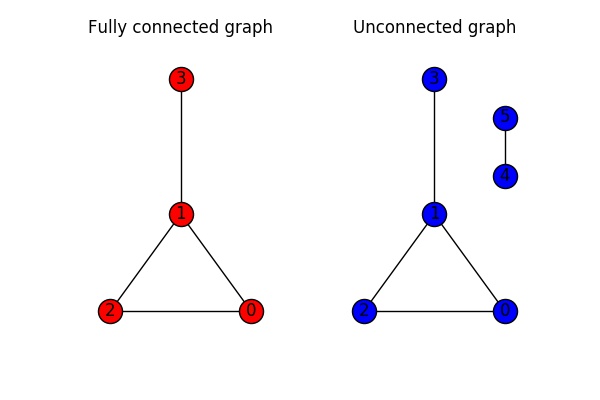
An undirected graph is called connected if there is a path between every pair of distinct
vertices of the graph.
An undirected graph that is not connected is called disconnected.
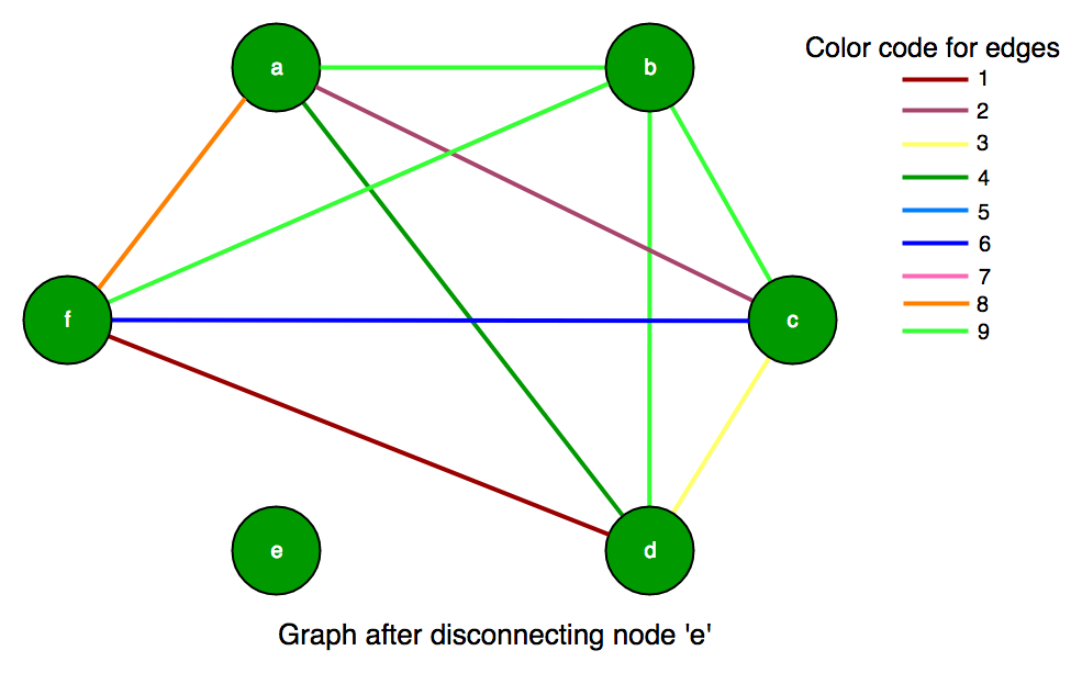
We say that we disconnect a graph when we remove vertices or edges, or both, to produce a
disconnected subgraph.
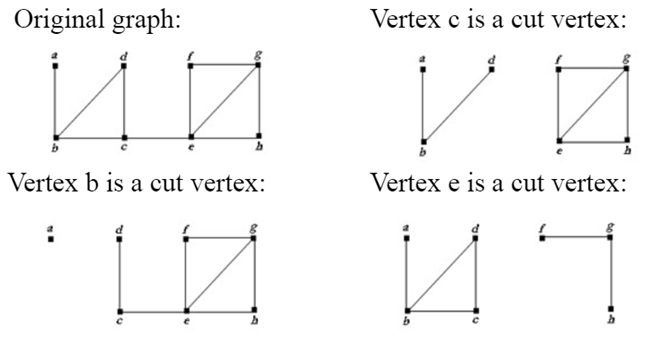
Cut vertices or Articulation points is the vertices that if they and their incident edges are removed from a graph, a subgraph with more connected components is produced.
An edge whose removal produces a graph with more connected components than in the original graph is called a Cut edge or Bridge.
The vertices b, c, e is cut vertices and the edge (c, e) is cut edge (javatpoint)
Vertex Connectivity
When a complete graph $K_n$ removes a vertex and all incidents to it, the resulting graph is a complete graph $K_{n-1}$ which also a connected graph.
Remove a vertex from a $K_6$ makes a $K_5$ graph (geeksforgeeks)
Connected graph having no cut vertex is a nonseparable graph which is more connected than a graph with a cut vertex.
A subset $V'$ of the vertex set $V$ of $G=(V,E)$ is a vertex cut, or separating set, if $G-V'$ is disconnected.
Vertex connectivity of a noncomplete graph $G$, denoted by $\kappa(G)$, is the minimum number of vertices in a vertex cut.
The Vertex connectivity is 1, because removing the vertex A makes 2 connected components (stackexchange)
When $G$ is a complete graph, it has no vertex cuts. Because removing any vertex and its incident edges still leaves a complete graph.
So, it’s impossible to define $\kappa(G)$ as the smallest number of vertices in a vertex cut when $G$ is complete. In this case, we define $\kappa(K_n) = n-1$ as the number of vertices needed to be removed to produce a graph with a single vertex.
In conclusion, for every graph G, $\kappa(G)$ is the minimum number of verties that can be removed from graph to either:
Disconnect G or
Prduce a graph with a single vertex
We have:
$0 \le \kappa(G) \le n-1$ if G has n vertices
$\kappa(G) = 0$ if and only if G is disconnected or $G = K_1$
$\kappa(G) = 1$ if and only if G is complete
The larger k(G) is, the more connected G is:
Disconnected graph or $K_1$ have $\kappa(G) = 0$
Connected graph with cut vetices and $K_2$ have $\kappa(G) = 1$
Graph without cut vertices and $K_3$ have $\kappa(G) = 2$
so on …
A graph is k-connected or k-vertex-connected if $\kappa(G) \ge k$:
1-connected graph if it is connected and not a graph containing a single vertex
2-connected is also called biconnected that is non seperable and has at least three vertices
G is a k-connected graph, then G is a j-connected for all j with $0 \le j \le k$
Edge Connectivity
A set of edge E' is called an edge cut of G if the subgraph $G - E'$ is disconnected.
The edge connectivity of a graph G, denoted $\lambda(G)$, is the minimum number of edges in an edge cut of G.
We always define $\lambda(G)$ for any connected graphs with at least one vertex because it is always possible to disconnect a graph by removing all edges incident to one of its vertices.
$\lambda(G) = 0$ if G is not connected.
If G is a graph with $n$ vertices, then $0 \le \lambda(G) \le n - 1$
$\lambda(G) = n - 1$ if and only if $G = K_n$
$\lambda(G) \le n - 2$ if and only if G is not a complete graph.
When $G = (V,E)$ is a noncomplete connected graph with at least three vertices:
$$\kappa(G) \le \lambda(G) \le \min_{v \in V} \deg(v) $$
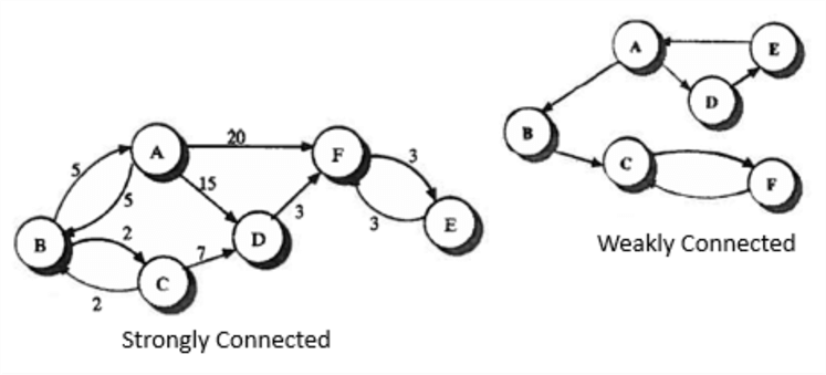
A directed graph is strongly connected if there is a path from a to b and from b to a whenever a and b are vertices in the graph.
A directed graph is weakly connected if there is a path between every two vertices in the underlying undirected graph.
A directed graph is weakly connected if and only if there is always a path between two vertices when the directions of the edges are disregarded. Clearly, any strongly connected directed graph is also weakly connected.
Strong connected and Weakly connected graph (mssqltips)
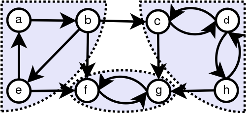
The strongly connected components or strong components of $G$ are the maximal strongly connected subgraphs which is the subgraphs of a directed graph $G$ that are strongly connected but not contained in larger strongly connected subgraphs.
Graph with strongly connected components marked (Wikipedia)
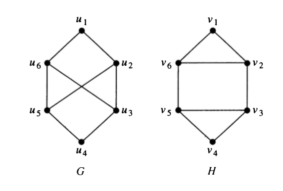
Both $G$ and $H$ have same three invariants: number of vertices, number of edges, and degrees of vertices—all agree for the two graphs.
However, $H$ has a simple circuit of length three, namely, $v_1, v_2, v_6, v_1$, whereas $G$ has no simple circuit of length three, as can be determined by inspection (all simple circuits in $G$ have length at least four). Because the existence of a simple circuit of length three is an isomorphic invariant, $G$ and $H$ are not isomorphic.
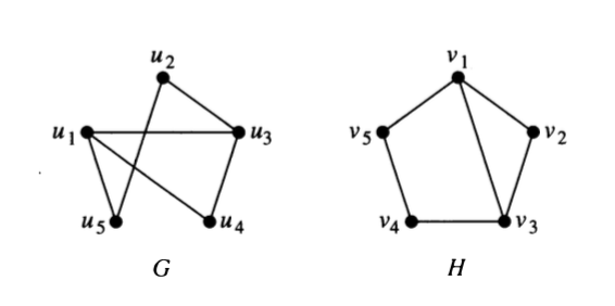
Both G and H have five vertices and six edges, both have two vertices of degree three and three vertices of degree two, and both have a simple circuit of length three, a simple circuit of length four, and a simple circuit of length five. Because all these isomorphic invariants agree, G and H may be isomorphic.
To confirm isomorphism, find the path go through all same degrees of 2 graphs. For example, the paths $u_1 \rightarrow u_4 \rightarrow u_3 \rightarrow u_2 \rightarrow u_5$ in $G$ and $v_3 \rightarrow v_2 \rightarrow v_1 \rightarrow v_5 \rightarrow v_4$ in $H$ both go through degrees: $3 \rightarrow 2 \rightarrow 3 \rightarrow 2 \rightarrow 2$. So, we can establish a mapping $f$ with $f(u_1) = v_3$, $f(u_4) = v_2$, $f(u_3) = v_1$, $f(u_2) = v_5$, and $f(u_5) = v_4$, this leads to that $G$ and $H$ are isomorphic.
Counting Paths Between Vertices
Let G be a graph with adjacency matrix $A$ with respect to the ordering $v_1, v_2, \dots, v_n$ of the vertices of the graph (with directed or undirected edges, with multiple edges and loops allowed).
The number of different paths of length $r$ from $v_i$ to $v_j$, where $r$ is a positive integer, equals the $(i, j)$th entry of $A^r$.
An Euler circuit in a graph G is a simple circuit containing every edge of G.
An Euler path in G is a simple path containing every edge of G.
Euler circuit and Euler path (Credit: github/memr5)
A connected multigraph with at least two vertices has an Euler circuit if and only if each of its vertices has even degree.
A connected multigraph has an Euler path but not an Euler circuit if and only if it has exactly two vertices of odd degree.
This is the recursive procedure to find the Euler path of a graph:
procedure FindEulerPath(V)
  1. iterate through all the edges outgoing from vertex V;
       remove this edge from the graph,
       and call FindEulerPath from the second end of this edge;
  2. add vertex V to the answer.
The procedure could be rewrite in the non-recursive version:
stack St;
put start vertex in St;
until St is empty
  let V be the value at the top of St;
  if degree(V) = 0, then
    add V to the answer;
    remove V from the top of St;
  otherwise
    find any edge coming out of V;
    remove it from the graph;
    put the second end of this edge in St;
An Euler circuit in a graph G is a simple circuit containing every edge of G.
An Euler path in G is a simple path containing every edge of G.
Euler circuit and Euler path (Credit: github/memr5)
A connected multigraph with at least two vertices has an Euler circuit if and only if each of its vertices has even degree.
A connected multigraph has an Euler path but not an Euler circuit if and only if it has exactly two vertices of odd degree.
This is the recursive procedure to find the Euler path of a graph:
procedure FindEulerPath(V)
  1. iterate through all the edges outgoing from vertex V;
       remove this edge from the graph,
       and call FindEulerPath from the second end of this edge;
  2. add vertex V to the answer.
The procedure could be rewrite in the non-recursive version:
stack St;
put start vertex in St;
until St is empty
  let V be the value at the top of St;
  if degree(V) = 0, then
    add V to the answer;
    remove V from the top of St;
  otherwise
    find any edge coming out of V;
    remove it from the graph;
    put the second end of this edge in St;
A simple path in a graph $G$ that passes through every vertex exactly once is called a Hamilton path, and a simple circuit in a graph G that passes through every vertex exactly once is called a Hamilton circuit.
That is, the simple path $x_0, x_1, \dots ,x_{n−1}, x_n$ in the graph $G = (V , E)$ is a Hamilton path if $V = {x_0, x_1, \cdots , x_{n−1}, x_n}$ and $x_i = x_j$ for $0 \le i < j \le n$, and the simple circuit $x_0, x_1, \dots , x_{n−1}, x_n, x_0$ (with $n > 0$) is a Hamilton circuit if $x_0, x_1, \dots , x_{n−1}, x_n$ is a Hamilton path.
There are no known simple
necessary and sufficient criteria for the existence of Hamilton circuits. However, many theorems are known that give sufficient conditions for the existence of Hamilton circuits. Also, certain properties can be used to show that a graph has no Hamilton circuit.
Dirac's theorem
If $G$ is a simple graph with n vertices with $n \ge 3$ such that the degree of every vertex in $G$ is at least $n/2$, then $G$ has a Hamilton circuit.
Ore's Theorem
If $G$ is a simple graph with $n$ vertices with $n \ge 3$ such that \deg(u) + \deg(v) \ge n for every pair of nonadjacent vertices $u$ and $v$ in $G$, then $G$ has a Hamilton circuit.
Shortest-Path Problems
Planar Graphs
Graph Coloring
]]>Huy PhamFundamentals of Unconstrained Optimization2018-11-11T00:00:00+00:002018-11-11T00:00:00+00:00https://pnhuy.github.io/optimization/2018/11/11/Fundamental-of-Unconstrained-OptimizationIn unconstrained optimization, we minimize an objective function that depends on real variable, with no restriction:
\[\min_{x} f(x)\]
where $x \in \mathbb{R}^n$ is a real vector with $n \ge 1$ components and $f: \mathbb{R}^n \rightarrow \mathbb{R}$ is a smooth function.
What is a solution?
A point $x*$ is a global minimizer if $f(x^*) \le f(x), \forall x \in \mathbb{R}^n$
The global minimizer can be difficult to find. And most algorithms are able to find only a local minimizer:
A point $x*$ is a local minimizer if there is a neighborhood N of $x*$ such that $f(x^*) \le f(x), \forall x \in N$
This is sometimes called a weak local minimizer.
A point $x*$ is a strict local minimizer (also called a strong local minimizer) if there is a neighborhood N of $x*$ such that $f(x^ *) < f(x), \forall x \in N$ with $x \ne x^ *$.
A slightly more exotic type of local minimizer:
A point $x*$ is an isolated local minimizer if there is a neighborhood N of $x*$ such that $x*$ is the only local minimizer in N.
While strict local minimizers are not always isolated, it is true that all isolated local minimizers are strict.
Recognizing a local minimum
Is x* is a local minimum? → Examine all the points in its immediate vicinity to make sure that none of them has a smaller function value.
If f is twice continuously differentiable, we may be able to tell that x* is a local minimizer (and possibly a strict local minimizer) by examining just the gradient $\nabla f(x^ * )$ and the Hessian $\nabla^2 f(x^ * )$ by using Taylor’s theorem.
Taylor's Theorem
Suppose that $f: \mathbb{R}^2 \rightarrow \mathbb{R}$ is continuously differentiable and that $p \in \mathbb{R}^n$. Then we have that
$$f(x+p) = f(x) + \nabla f(x+tp)^Tp$$
for some $t \in (0,1)$.
Moreover, if $f$ is twice continuously differentiable, we have that
$$\nabla f(x+p) = \nabla f(x) + \int_0^1 \nabla ^2 f(x+tp)p \mathrm{d}t$$
and that
$$f(x+p) = f(x) + \nabla f(x+tp)^Tp +\frac{1}{2}p^T \nabla ^2 f(x+tp)p$$
Necessary conditions for optimality are derived by assuming that x* is a local minimizer and then providing facts about $\nabla f(x^ * $ and $\nabla^2 f(x^ * )$.
First-Order Necessary Conditions
If x* is a local minimizer and f is continuous differentiable in an open neighborhood of x* , then $\nabla f(x^*) = 0$.
Second-Order Necessary Conditions
If x* is a local minimizer of $f$ and $\nabla^2 f$ is continuous in an open neighborhood of x* , then $\nabla f(x^ * ) = 0$ and $\nabla^2 f(x^*)$ is positive semidefinite.
Second-Order Sufficient Conditions
Suppose that $\nabla^2 f$ is continuous in an open neighborhood of x* and that $\nabla f(x^ * ) = 0$ and $\nabla^2 f(x^ * ) $ is positive definite. Then x* is a strict *local minimizer* of $f$.
When f is convex, any local minimizer x* is a global minimizer of f. If in addition f is differentiable, then any stationary point x* is a global minimizer of f.
Algorithms
Line Search vs Trust Region
General approach of algorithms for unconstrained minimization:
Supply a starting point $x_0$
Generate a sequence of iterates ${x_k}_{k=0}^\infty$
Terminate when either no more progress can be made or when it seems that a solution point has been approximated with sufficient accuracy.
There are 2 common strategies for moving from the current point $x_k$ to a new iterate $x_{k+1}$: Line search and Trust region.
Line search strategy
Choose a direction $p_k$
Search along this direction from the current state $x_k$ for a new state with a lower function value
The distance can be found by solving approximately ($\alpha$ is step length):
\[\min_{\alpha>0} f(x_k + \alpha p_k)\]
The exact minimization is expensive and unnecessary. In fact, the line search algorithm generates a limited number of trial step lengths until it finds one that the loosely approximates the minimum of above minimization.
Trust region strategy
Construct a model function $m_k$ that approximately similar to $f$ in neighborhood of $x_k$.
Search minimizer of $m_k$ (also $x_k$) in some region around $x_k$. In other words, we find the candidate step p by approximately solving the following subproblem:
\[\min_{p} m_k(x_k+p)\]
where $x_k +p$ lies inside the trust region.
If solution does not produce a sufficient decrease in $f$ → Trust region is too large → Shrink it and re-solve.
The trust region is defined by $|p|_2 \le \Delta$ where the scalar $\Delta > 0$ is called the trust-region radius. The model $m_k$ is usually defined to be a quadratic function of the form:
where $f_k, \nabla f_k, B_k$ are a scalar, vector, matrix, respectively. $B_k$ is either the Hessian $\nabla^2 f_k$ or some approximation to it.
The line search and trust region approaches differ in the order in which they choose the direction and distance of the move to the next iterate.
For line search, fixing the direction $p_k$ → identifying an appropriate distance $\alpha_k$
For trust region, choose a maximum distance - the trust region radius $\Delta_k$ → seek a direction and step
Search directions for Line search methods
The steepest-descent direction
The most obvious choice for search direction for line search method is the steepest-descent direction $- \nabla f_k$. That means among all the directions we could move from $x_k$, this is the way that $f$ decreases most rapidly.
Let’s prove this. By Taylor’s theorem, we have
\[f(x_k +\alpha p) = f(x_k) +\alpha p^T \nabla f_k + \frac{1}{2} \alpha^2 p^T \nabla^2 f(x_k + tp) p \text{, for some }t \in (o, \alpha)\]
which p is the search direction and $\alpha$ is the step-length parameter.
So, in this formula, the rate of change in $f$ along the direction $p$ at $x_k$ is $p^T \nabla f_k$.
As the result, the unit direction $p$ of the most rapid decrease is the solution to the problem
\[\min_p p^T \nabla f_k \text{, subject to } \|p\| =1\]
Because $p^T \nabla f_k = |p| | \nabla f_k | \cos \theta$ and $| p|=1$, we have $p^T \nabla f_k = | \nabla f_k | \cos \theta$. Minimization in (9) occurs when $\cos \theta = -1$ at $\theta = \pi$. In other words, the solution to (9) is
\[p = -\nabla f_k / \|\nabla f_k\|\]
In visual representation, this direction is orthogonal to the contours of the function.
Advantage of the steepest descent direction is that it require calculation of the gradient $\nabla f_k$ but not of second derivatives. However, it can be excruciatingly slow on difficult problems.
When the $\theta$ is not exactly $\pi$ or the direction is just descent, Taylor’s theorem also verifies that $f$ is still decreased with a sufficiently small. In this situation, $p_k$ is a down hill direction.
Newton direction
From the second-order Taylor series approximation to $f(x_k + p)$ :
Assuming that $\nabla^2 f_k$ is positive definite, the Newton direction is defined by finding the vector $p$ that minimizes $m_k (p)$. By simply setting the derivative of $m_k(p)$ to zero, we obtain the following explicit formula:
\[p^N_k = -\nabla^2 f_k^{-1} \nabla f_k\]
When $\nabla^2 f_k$ is positive definite, we have
\[\nabla f_k^T p_k^N = -p_k^{NT} \nabla^2 f_k p_k^N \le -\sigma_k \| p_k^N \|^2 \text{, for some }\sigma_k > 0\]
Unless the gradient $\nabla f_k$ is zero, we have that $\nabla f_k^T p_k^N < 0 $, so the Newton direction is a descent direction.
Unlike the steepest descent direction, there is a “natural” step length of 1 associated with the Newton direction. Most line search implementations of Newton’s method use the unit step $\alpha = 1$ where possible and adjust this step length only when it does not produce a satisfactory reduction in the value of $f$.
When $\nabla^2 f_k$ is not positive definite, the Newton direction may not even be defined, since $\nabla^2 f_k^{-1}$ may not exist. Even when it is defined, it may not satisfy the descent property $\nabla f_k^T p_k^N < 0$. So that, it is unsuitable as a search direction.
In these cases, $p_k$ need to be changed to guarantee the downhill condition while keeping the benefit of second-order information in $\nabla^2 f_k$.
The Newton direction approach has a fast rate of local convergence - quadratic.
The main disadvantage of the Newton direction is the need for the Hessian $\nabla^2 f(x)$. This is usually a cumbersome, error-prone and expensive process.
Quasi-Newton direction
This method do not require computation of the Hessian but still have a super linear rate of convergence.
They use an approximation $B_k$ for the true Hessian $\nabla^2 f_k$. In this case, $B_k$ is updated to take account of the additional knowledge gained after each step. The updates make use of the fact that changes in the gradient $g$ provide information about the second derivative of $f$ along the search direction.
Because $\nabla f(.)$ is continuous, the size of final integral term is $o(|p|)$. By setting $x = x_k$ and $p = x_{k+1} - x_k$:
\[
\nabla f_{k+1} = \nabla f_k + \nabla^2 f_{k+1} (x_{k+1} - x_k) + o(| x_{k+1} - x_k |)
\]
When $x_k$ and $x_{k+1}$ lie nearly the solution $x*$, within which $\nabla f$ is positive definite, the final term in this expansion is eventually dominated by the $\nabla^2 f_k (x_{k+1} - x_k)$ and $\nabla^2 f_{k+1} (x_{k+1} - x_k) \approx \nabla f_{k+1} - \nabla f_k$
We choose the new Hessian approximation $B_{k+1}$ so that it mimics this property. This means that it needs to satisfy the secant equation:
\[
B_{k+1} s_k = y_k
\]
where
\[
s_k = x_{k+1} - x_k, y_k = \nabla f_{k+1} - \nabla f_k
\]
There are two most popular way to choose $B_{k+1}$:
The BFGS (Broyden-Fletcher-Goldfarb-Shanno) formula (which is a rank-two matrix):
\[
B_{k+1} = B_k - \frac{B_k s_k s_k^T B_k}{s_k^T B_k s_k} + \frac{y_k y_k^T}{y_k^T s_k}
\]
The quasi-Newton search direction is $p_k = -B_k^{-1} \nabla f_k$
By applying the inverse approximation $H_k \overset{def}{=} B_k^{-1}$, the above formula is equivalent to
\[
H_{k+1} = (I - \rho_k s_k y_k^T) H_k (I - \rho_k y_k s_k^T) + \rho_k s_k s_k^T, \rho_k = \frac{1}{y_k^T s_k}
\]
This can be implemented as a matrix-vector multiplication, which is typically simpler than the previous formula.
Nonlinear conjugate gradient methods
This method of search direction has form
\[
p_k = -\nabla f(x_k) + \beta_k p_{k-1}
\]
where $\beta_k$ is a scalar that ensure that $p_k$ and $p_{k-1}$ are conjugate.
This method is much more effective than the steepest descent direction, not requiring storage of matrices and simple to compute but does not retain the fast convergence rates of Newton or quasi-Newton methods.
Models for Trust-region methods
The subproblem of Trust-region is
\[\min_{p} m_k(x_k + p)\]
where $x_k + p$ lies inside the trust region.
The model function has the quadratic fuction form:
We set $B_k = 0$ and define the trust region using the Euclidean norm, the trust region subproblem becomes
\[
\min_{p} f_k + p^T \nabla f_k \text{, subject to }| p |_2 \le \Delta_k
\]
We can write the solution to this problem in closed form as
\[
p_k = -\frac{\Delta_k \nabla f_k}{| \nabla f_k |}
\]
This is simply a steepest descent step in which the step length is determined by the trust-region radius; the trust-region and line search approaches are essentially the same in this case.
We can choose $B_k$ to be exact Hessian $\nabla^2 f_k$ in quadratic model. The subprolem is guaranteed to have a solution $p_k$ even though the $\nabla^2 f_k$ is not positive definite because of the restriction $| p|_2 \le \Delta_k$.
We are also able to choose $B_k$ by means of a quasi-Newton approximation. This is trust-region quasi-Newton method.
Scaling
A uncontrained optimization is poorly scaled if changes to x in a certain direction prodct much larger variations in the value of $f$ than do changes to x in another direction.
Steepest descent and som optimization algorithms are sensitive to poor scaling, while others such as Newton’s method are unaffected by it.
In design complete algorithms, scale invariance is included in all aspects of algoritm. In general, it is easier to preserve scale invariance for line search algorithms than for trust-region algorithms.
Rates of convergence
Let $\{x_k\}$ be a sequence in $\mathbb{R}^n$ that converges to $x^{*}$.
We say that the convergence is Q-linear if there is a constant $r \in (0,1)$ such that
$$\frac{\| x_{k+1} - x* \|}{\| x_k - x* \|} \le r \text{, for all k sufficiently large}$$
The convergence is said to be Q-superlinear if
$$\lim_{k \rightarrow \infty} \frac{\| x_{k+1} - x* \|}{\| x_k - x* \|} = 0 \text{, for all k sufficiently large}$$
Q-quadratic is optained if
$$\frac{\| x_{k+1} - x* \|}{\| x_k - x* \|^2} \le M \text{, for all k sufficiently large}$$
In general, the Q-order of convergence is p (with p > 1) if there is a positive constant M such that
$$\frac{\| x_{k+1} - x* \|}{\| x_k - x* \|^p} \le M \text{, for all k sufficiently large}$$
For example:
$1+(0.5)^k$ converges Q-linearly to 1
$1+k^{-k}$ converges superlinearly to 1
$1+ (0.5)^{2^k}$ converses quadratically to 1
The speed of convergence depends on $r$ and $M$. These values depend on both algorithms and properties of problem. However, a quadratically convergent sequence will always eventually converge faster than a linearly convergent sequence.
Quasi-Newton methods typically converge Q-superlinearly, whereas Newton’s method converges Q-quadratically. In contrast, steepest descent algorithms converge only at a Q-linear rate, and when the problem is ill-conditioned the convergence constant $r$ is close to 1.
]]>Huy PhamHow To Choose Data Visualization Techniques2018-07-19T00:00:00+00:002018-07-19T00:00:00+00:00https://pnhuy.github.io/2018/07/19/How-to-choose-data-visualization-techniques
]]>Huy PhamIntroduction to Machine learning2018-07-17T00:00:00+00:002018-07-17T00:00:00+00:00https://pnhuy.github.io/machinelearning/2018/07/17/Fundamental-Machine-LearningFour branches of machine learning
Supervised learning
It consists of learning to map input data to known targets:
$f: x (input) \rightarrow y (output)$
There are 2 major techniques in supervised: classification and regression, and there are more exotic variants as well:
Sequence generation, eg: captioning the picture
Syntax tree prediction, eg: decomposition a sentence
Object detection, eg: draw a bounding box aroung certain objects inside a picture
Image segmentation, eg:..
Unsupervised learning
It consists of finding interesting transformations of the input data without targets.
Application of unsupervised learning is supports in data visualization, data compression or data denoising or to better understanding the correlation present in the data.
Well-known categories of unsupervised learning are Dimensionality reduction and clustering
Self-supervised learning
It is supervised learning without human-annotated labels, they’re generated from the input data, typically using a heuristic algorithms
Well-knowns instance of self-supervised learning: autoencoders
Reinforcement learning
An agent receives information about its environment and learns to choose actions that will maximize some reward. Some potential application area of reinforcement learning: self-driving cars, robotics, resource management, education,…
Evaluating machine learning models
In machine learning, the main goal is to archive models that generalize (perform well on never-before-seen data) and overfitting is the central obstacle. There are some strategies to measure generalization or evaluate machine-learning models.
Training, validation and test sets
The data set is divided into THREE sets:
Training set: train the model
Validation set: evaluate the model
Test set: test the model
The model developing always involves tuning its configuration, eg:
The number of layers
The size of layers
other hyperparameters…
Tuning the configuration can result in the overfitting to the validation set because of information leaks. Every time you tune a hyperparameter of the model based on the model’s performance on the validation set, some information about the validation data leaks into the model. At the end, the model performs well on the validation data, so you need to use a completely differet dataset to evaluate the model: the test dataset.
There are some methods for validation:
Simple hold-out validation
K-fold validation
Iterated K-fold validation with shuffling
It consists of applying K-fold validation multiple times and shuffling the data every time before splitting it K ways.
Notes
Data representativeness: you should randomly shuffle your data before splitting it to make sure that the training set and test set could be representative of the whole data.
Time series data should not randomly shuffle, the test set should be posterior to the data in the training set.
Redundancy in your data
Data preprocessing, feature engineering, and feature learning
Data preprocessing
Aim: making the raw data more amenable (easy to control) to neural networks.
Vectorization
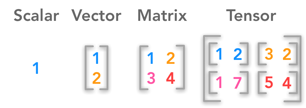
Inputs or targets in a neural network must be tensors of floating-point data (or integers).
If your data is sound, images, text, you should first turn into tensors. This step called data vectorization.
Value normalization
In general, it isn’t safe to feed the neural networks data that takes relatively large values or data the is heterogeneous (one feature is in the range 0-1, one feature is in the range 100-200).
This causes large gradient updates that will prevent the network from converging. To make learning easier for your network, your data should have the following characteristics:
Take small values
Be homogenous
The normalization (to mean of 0 and standard deviation of 1) is the common practice.
Handling the missing values
In general, with neural networks, it’s safe to input missing values as 0, with the condition that 0 isn’t already a meaningful value. The network will learn from exposure to the data that the value 0 means missing data and will start ignoring the value.
Feature engineering
The essense of feature engineering is making a problem easier by expressing it in a simpler way. It usually requires understanding the problem in depth.
Example:
Raw data: Pixel gird of clock -> Better feature: clock hands’ coordinates {x1, y2}, {x2, y2} -> Even better features: angles of clock hands theta1, theta 2
Good features allow you to solve problems more elegantly while using fewer resources. For instance, it would be ridiculous to solve the problem of reading a clock face using a convolutional neural network.
Good features let you solve a problem with far less data. The ability of deep
Overfitting and Underfitting
The fundamental issue in machine learning is the tension between optimization and generalization.
Optimization: adjusting a model to get the best performance possible on the training data.
Generalization: how well the trained model performs on data it has never seen before.
At the beginning of training: optimization and generalization are correlated: the lower the loss on training data, the lower the loss on test data. While this is happening, your model is said to be underfit -> there is still progress to be made; the network hasn’t yet modeled all relevant patterns in the training data.
After a certain number of iterations on the training data, generalization stops improving and validation metrics stall and then begin to degrade: the model is starting to overfit -> it’s beginning to learn patterns that are specific to the training data but that are misleading or irrelevant when it comes to new data.
Get more training data is usually useful: a model trained on more data will naturally generalize better.
If more data failed, the next solution is to modulate the quantity of information that your model is allowed to store or to add constraints on what information it’s allowed to store. -> regularization.
Reducing the network’s size
This is the simplest way to prevent overfitting.
The network’s size or The number of learnable paramaters in a model (determined by the number of layers and the number of units per layer) is often referred to as the model’s capacity. A model with more parameters has more memorization capacity, so it can easily learn a perfect dictionary-like mapping between training samples and their targets - a mapping with out any generalization power.
Deep learning models tend to be good at fitting to the training data, but the real challenge is generalization.
The model should have just enough parameters that they don’t underfitting.
No formula to determine the right number of layers or the right size of each layer. Need to research to find the optimal model size of your data.
Adding weight regularization
This way to mitigate overfitting is to put constraints on the complexity of a network by forcing its weights to take only small values, which makes the distribution of weight values more regular => weight regularization
There are 2 flavors:
L1 regularization -> The cost added is proportional to the absolute value of the weight coefficients (L1 norm of the weights)
L2 regularization -> The cost added is proportional to the square of the value of the weight coefficients (L2 norm of the weights/ Weight decay)
Adding dropout
Dropout is one of the most effective and most commonly used regularization techniques for neural networks.
When apply to a layer,dropout consists of randomly dropping out (setting to zero) a number of output features of the layer during training.